2. User Guide

2.1. Set up

2.1.1. Requirements

AftFore depends on the following external packages:

• Python 2.7
• Numpy
• Scipy
• Matplotlib
• Pandas

Please see Installing the SciPy Stack for installing Numpy, Scipy, and Matplotlib.

2.1.2. Download

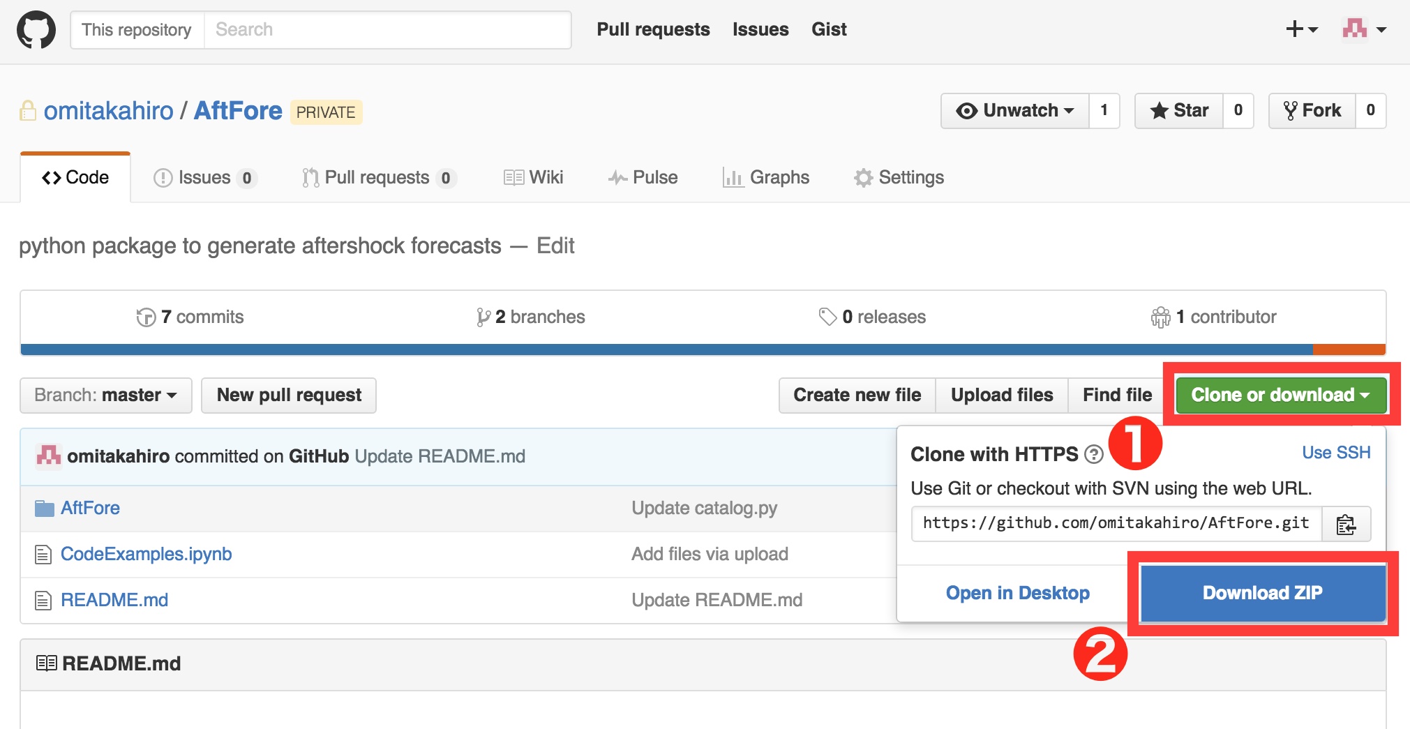
A souce code is available at https://github.com/omitakahiro/AftFore/.

Please see the below figure to download the zipped source file. After unzipping the downloaded file, please put the AftFore folder (in the unzipped folder) to your working directory.

2.2. Data Preparation

A data file is an ascii file that contains the list of the relative time after the main shock [day] (the first column) and magnitude (the second column) of the main shock and its aftershocks. The first event is identified as the main shock, and the time of the main shock must be set to 0. A sample aftershock data of the 1995 Kobe earthquake of M7.3 is included in the source file (./AftFore/Kobe.txt).

Note

AftFore uses all the aftershock data including earthquake with magnitude smaller than the completeness magnitude for the estimation, so please inclue all the available data in your data file.

A data file is like:

0.000000 7.3
0.001652 4.4
0.001890 4.2
0.002048 4.5
0.002455 5.2
0.002933 3.8
0.003422 4.2
0.003651 4.0
0.004033 3.3
0.004396 5.0
0.005003 3.6
0.005305 3.8
0.012113 3.2
0.012714 3.1
0.012822 3.8
...

2.3. Program Workflow

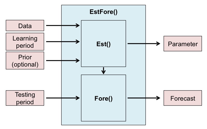
The forecast procedure consists of two steps.

1. The model parameters are estimated from the aftershock data in the learning period, done by a function Est(). We here use the prior probability distribution for the Bayesian estimation, which is set to be the default values used in Omi et al., (2016) unless otherwise set.
2. The forecast for the testing period is produced based on the estimated parameter sets, done by a function Fore().

A function EstFore() performs the both two tasks and provides a simple way to produce the forecasts. If the user just wants to generate a forecast, EstFore() is enough. The user may use Est() or Fore() for the advanced purpose.

2.4. Quick Start

Note

Before running the code, the user needs to (1) put the downloaded AftFore folder in your working directory and (2) prepare the data file.

The below code shows the simplest way to generate a forecast by using EstFore(). The parameters that the user has to set are t_learn (the range of the learning period), t_test (the range of the testing period), and Data (the path of the data file). For example, this code uses the data file ‘./AftFore/Kobe.txt’ and generates a forecast for the testing period [1.0, 2.0] (day) based on the data in the learning period [0.0, 1.0] (day). The estimation is carried out with the default prior probability distribution. See prior for a method to customize the prior.

import AftFore as aft

t_learn = [0.0, 1.0]            # The range of the learning period [day].
t_test  = [1.0, 2.0]            # The range of the testing period [day].
Data    = './AftFore/Kobe.txt'  # The path of the date file

aft.EstFore(Data, t_learn, t_test)

This process takes about a few minutes. The forecast result (the number of earthquakes with \(M>M_t\) in the testing period, and the probability to have at least one earthquake with \(M>M_t\) in the testing period) is saved in fore.txt.

# (M_t) (expected_number) (lower bound of 95% interval) (upper bound of 95% interval) (probability)
0.95         682.218         564         832      1.0000
1.05         576.029         477         699      1.0000
1.15         486.368         403         589      1.0000
1.25         410.664         340         496      1.0000
1.35         346.743         287         419      1.0000
1.45         292.772         241         354      1.0000
1.55         247.201         202         300      1.0000
1.65         208.723         170         255      1.0000
1.75         176.235         142         217      1.0000
1.85         148.804         119         185      1.0000
1.95         125.642          99         158      1.0000
2.05         106.085          82         135      1.0000
...

EstFore() also generates files, param.pkl, param.pdf, and fore.pdf. See Generated Files for the details.

Note

EstFore() may raise some warnings, but the user does not have to care about this for the most cases.

2.5. Code Examples

The user needs to import AftFore at first before running the following examples.

import AftFore as aft

2.5.1. Parameter Estimation

The parameter estimation is carried out by Est(). Here the estimation is carried out under the defalut prior probability distribution. See prior for a method to customize the prior.

t_learn = [0.0, 1.0]            # The range of the learning period [day].
Data    = './AftFore/Kobe.txt'  # The path of the date file

param = aft.Est(Data, t_learn)

Est() returns a parameter object param that contains the estimated parameter values and other information, which will be used for producing forecasts. Est() also generates: param.pkl (a pickle file that saves param) and param.pdf (a figure summarizing the estimated parameters).

The param can be loaded from param.pkl.

import pickle

param = pickle.load(open('param.pkl','rb'))

2.5.2. Forecast Generation

The forecast is produced using the estimated parameter sets param by Fore().

t_test  = [1.0, 2.0]            # The range of the testing period [day].

aft.Fore(param, t_test)

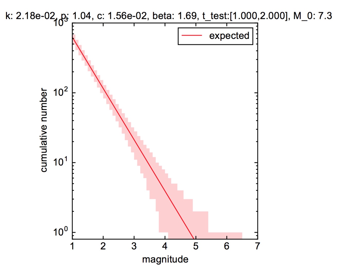
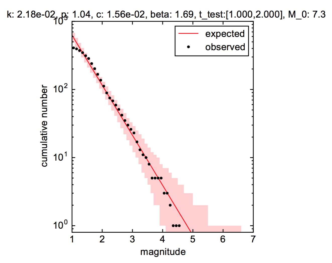
Fore() generates fore.txt and fore.pdf that summarize the forecast result.

The user may want to compare the forecast with the observation. By setting a keyword Data_test to the path of the data file, the observation in the testing period is plotted in fore.pdf. See fore.pdf for the detail.

t_test  = [1.0, 2.0]             # The range of the testing period [day].
Data_test = './AftFore/Kobe.txt' # The path of the data file including the data in the testing period

aft.Fore(param, t_test, Data_test=Data_test)

2.6. Tips

2.6.1. How to extract the estimated parameter values

The estimated parameter values are stored in the object param["para"] (please see also param for the detail).

The MAP parameters:

[k,p,c,beta] = param["para"][["k", "p", "c", "beta"]]
print( "k: %f" % k )
print( "p: %f" % p )
print( "c: %f" % c )
print( "beta: %f" % beta )

""" OUTPUT
k: 0.021769
p: 1.037202
c: 0.015635
beta: 1.691913
"""

Please also see the next tips for forecasting the aftershock activity from these parameters.

2.6.2. How to calculate the estimation uncertainty

The sets of the parameters sampled from the posterior distribution is stored in the object param["para_mcmc"] (please see also param for the detail). The estimation uncertainty can be obtained by

print( param["para_mcmc"][["k", "p", "c", "beta"]].std() )

""" OUTPUT
k        0.008331
p        0.068125
c        0.006976
beta     0.071577
"""

2.6.3. How the parameter values are related to the earthquake occurrence rate or earthquake number

In our model, the occurrence rate of an aftershock of magnithde \(M\) at time \(t\) is given by

\[\lambda(t,M) = \frac{k}{(t+c)^p}\beta e^{-\beta(M-M_0)},\]

where \(M_0\) represents the mainshock magnitude.

For a given threshold magnitude \(M_{th}\), the occurrence rate of an aftershock of \(M>M_{th}\) at time \(t\) is obtained by

\[\lambda(t) = \frac{k}{(t+c)^p} e^{\beta(M_0-M_{th})}.\]

The expected number of aftershocks of \(M>M_{th}\) in the time interval \([t_1,t_2]\) is also obtained by

\[n = \int_{t_1}^{t_2}dt \lambda(t) = \frac{k}{-p+1} [(t_2+c)^{-p+1}-(t_1+c)^{-p+1}] e^{\beta(M_0-M_{th})}.\]

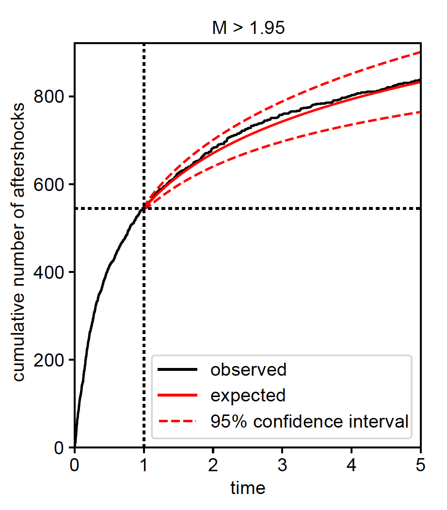
2.6.4. How to show the N-T plot (the cumulative number of aftershocks versus time), compared with the forecast (Experimental)

A function NT_plot() shows the time evolution of the cumulative number of aftershocks of M > mag_th in the time interval [0, t_test_end], compared with the forecast. The confidence interval is evaluated in a Bayesian way, using the parameter sets sampled from the posterior distribution (para_mcmc in param).

# parameter estimation
t_learn = [0.0, 1.0]            # The range of the learning period [day].
Data    = './AftFore/Kobe.txt'  # The path of the date file

param = aft.Est(Data, t_learn)

# showing the NT plot with the forecast
mag_th   = 1.95               # The magnitude threshold M_th fore forecasting
t_test_end  = 5.0             # The end of the forecasting period [day]. The time interval [0, t_test_end]

aft.NT_plot(Data, t_test_end, mag_th, param)

The output figure is saved as “NT.pdf”.

2.7. AftFore Reference

2.7.1. Function

AftFore.Est(Data, t_learn, prior=None)

Keywords:If prior is None, the default prior probability distribution is used for the estimation. See prior for a method to customize the prior. Returns:param Generates:param.pkl and param.pdf

AftFore.Fore(param, t_test, Data_test=None)

Keywords:If a keywrod Data_test is set to the path of the data file, the observation in the test period is added in the fore.pdf. Generates:fore.txt and fore.pdf

AftFore.EstFore(Data, t_learn, t_test, prior=None)

Keywords:If prior is None, the default prior probability distribution is used for the estimation. See prior for a method to customize the prior. Generates:param.pkl, param.pdf, fore.txt, and fore.pdf

2.7.2. Object

t_learn

[float, float]

The lower and upper range of the leraning period. The unit is ‘day’.

t_test

[float, float]

The lower and upper range of the testing period. The unit is ‘day’.

Data

string

The path of the data file

param

A parameter object. Also see How to extract the estimated parameter values and How to calculate the estimation uncertainty.

param[“para”]: the MAP estimated parameters (pandas.Series)

param[“para_mcmc”]: the parameter set sampled from the posterior distribution (pandas.DataFrame)

param[“mag_ref”]: the main shock magnitude

param[“t”]: the estimation period

prior

A prior object (optional: the default prior is used unless otherwise set)

The user can introduce the prior for the parameters {\(K,p,c,\beta,\sigma,\mu1\)} (Please see here for the detail of each parameter). A prior object is a list where each element defines the prior probability distribution of each parameter. A prior probability distribution of each parameter is specified by a list [para_name,prior_type,mu,sigma].

para_name: string

A name of the parameter (string) from {‘k’,’p’,’c’,’beta’,’sigma’,’mu1’}

para_type: string

A probability distribution function from the below list

‘n’: the normal distribution \(p(x)=\frac{1}{\sqrt{2\pi\sigma^2}}\exp[-\frac{(x-\mu)^2}{2\sigma^2}]\)

‘ln’: the log-normal distribution \(p(x)=\frac{1}{x\sqrt{2\pi\sigma^2}}\exp[-\frac{(\ln(x)-\mu)^2}{2\sigma^2}]\)

‘f’: the Dirac’s delta \(p(x)=\delta(x-\mu)\) (This prior fixes a given parameter to be \(\mu\))

mu: float

the \(\mu\)-value of the prior probability distribution function

sigma: float

the \(\sigma\)-value of the prior probability distribution function. Set sigma to 0, if ‘f’ is chosen for para_type.

For example, if the user want to use the normal distribution with \(\mu=2.0\) and \(\sigma=0.5\) as the prior of the parameter \(\beta\), the prior object is given as:

prior = [['beta','n',2.0,0.5]]

The user can introduce the prior for multiple parameters. The below code is the setting of the default prior.

import numpy as np
prior =[]
prior.append(['beta','n',0.85*np.log(10.0),0.15*np.log(10.0)])
prior.append(['p','n',1.05,0.13])
prior.append(['c','ln',-4.02,1.42])
prior.append(['sigma','ln',np.log(0.2),1.0])

Finally the prior object is passed to the keyword argument prior in Est() or EstFore().

aft.EstFore(Data,t_lean,t_test,prior=prior)

Note

When the user uses the customized prior, it is strongly recommended to introduce a prior for the \(\sigma\)-parameter for the computational stability. For example, the prior [‘sigma’,’ln’,np.log(0.2),1.0] is used for the \(\sigma\)-parameter in the default prior.

2.7.3. Generated Files

param.pkl

A pickle file that stores a parameter object param. See Parameter Estimation for the method to retrive param from the pickle file.

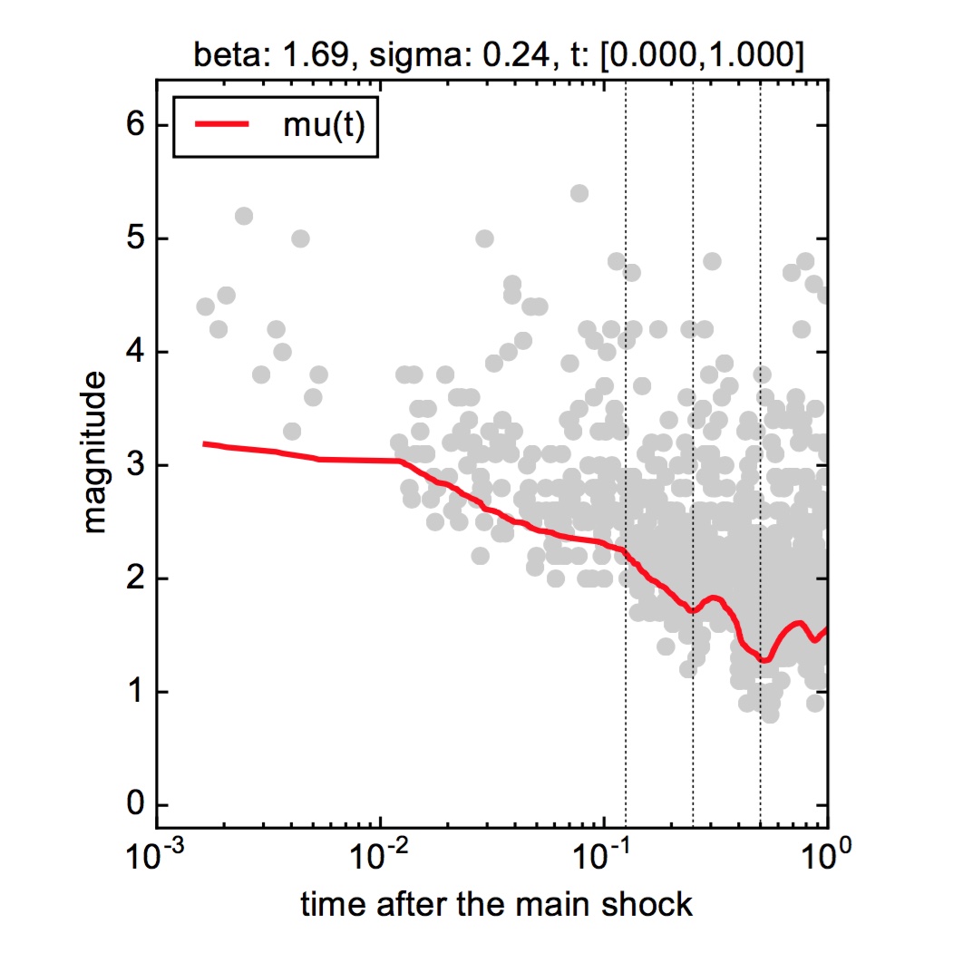
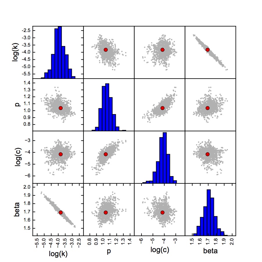
param.pdf

A figure showing (1) the MT plot superinposed with the time-varying magnitude of 50% detection rate and (2) the scatter plot matrix of the estimated parameter sets (red dots: MAP parameter values, gray dots: sampled parameter sets).

fore.txt

A list of the target magnitude \(M_t\), the expected number of earthquakes in the testing period with \(M>M_t\), its 95% confidencial interval, the probability to have at least one earthquake with \(M>M_t\) in the testing period.

# (M_t) (expected_number) (lower bound of 95% interval) (upper bound of 95% interval) (probability)
0.95         682.218         564         832      1.0000
1.05         576.029         477         699      1.0000
1.15         486.368         403         589      1.0000
1.25         410.664         340         496      1.0000
1.35         346.743         287         419      1.0000
1.45         292.772         241         354      1.0000
1.55         247.201         202         300      1.0000
1.65         208.723         170         255      1.0000
1.75         176.235         142         217      1.0000
1.85         148.804         119         185      1.0000
1.95         125.642          99         158      1.0000
2.05         106.085          82         135      1.0000
...

fore.pdf

A figure showing the forecast result.

If a keyword Data_test is set in Fore(), the observation in the testing period is added.